In mathematics, a
category
is a structure made of so-called objects and so-called morphisms from one object to another or the same object.
Two morphisms can be connected in series, if the target object of the first morphism is the source object of the second morphism.
The result is a morphism from the source object of the first morphism to the target object of the second morphism.
Additionally, for every object O there is an identity morphism (denoted in the following by | or \ or /)
from O to O itself that does not change other morphisms when composed with them in series.
Here I write the serial composition of morphisms by writing them one below the other:
  f
  g
  |
  h
is the same as
  f
  g
  h
That denotes a compound morphism from A to D, if we assume that f goes from A to B, g goes from B to C and h goes from C to D.
A well-known category is the one where the objects are data types and the morphisms are functions between these types. The serial composition corresponds to function composition, and the identity morphism is the function that returns its parameter unchanged. The following will be mainly about this category.
Another interesting category whose morphisms are not functions is the category whose morphisms are relations between data types.
In a monoidal category there is an additional operation: Composing morphisms (and Objects) side by side, called monoidal product or tensor product. The monoidal product must satisfy certain conditions, for example:
  |  |       |  g       f  |
  f  g   =   |  |   =   |  |
  |  |       f  |       |  g
These rules arise naturally from the used notation. The neutral element of the monoidal product is simply drawn as empty space. This kind of diagram is called string diagram.
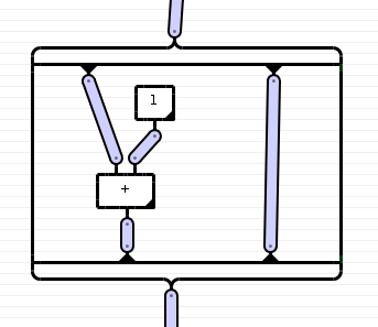
There are two important possibilities to equip the category of functions and data types with a monoidal product. The first possibility (that we will mainly consider in the following) is to interpret the monoidal product of data types as tuple formation. For two simple data types T and U, (T U) then is the Cartesian product T×U, and if the factors of the monoidal product are tuple types themselves, it is the concatenation of tuples; (T×U×V) (W×X) becomes (T×U×V×W×X). The monoidal product of functions is a function that takes a tuple, decomposes it into sub-tuples of the appropriate size, passes one to each of the factor functions and assembles the results into a single tuple again. With this, one may write data flow graphs like the following:
         |
    (3)  |
     |   |  (4)
      \ /    |
       +    /
       |   /
        \ /
         *
         |
It represents a function that increases its argument by 3 and multiplies it by 4. Here, (n) stands for the function that maps the empty tuple to the constant value n.
With the other possibility, the monoidal product of data types T and U is interpreted as disjoint union T ⊕ U of the data types. An element of (T U) is either an element of T together with the information that it belongs to the first factor, or it is an element of U with the information that it belongs to the second factor. The monoidal product of two functions is a function that uses one of the factor functions, depending on which of the factors of the input type the input value belong to. The corresponding string diagrams have a certain semantic similarity with control flow graphs. How to make loops in such a control flow graph I will tell further below.
Other interesting monoidal categories: The category of data types and relations can straightforwardly be equipped with a monoidal product. For the category of vector spaces and linear maps one can use either the tensor product or the direct sum as the monoidal product. If you take the tensor product, the string diagrams correspond to Penrose graphical notation.
Then there's the category of tangles, whose objects are natural numbers
and whose morphisms are tangles of strings.
The numbers count the strings that enter of exit the tangle.
A simple string, denoted by |, / or \, is the identity morphism of the object 1.
There are two elementary morphisms of the object 2 to itself: The braiding ,\´ and the inverse braiding `/..
These are supposed to depict two strings crossing over.
Then there are the morphism cup
, written \_/, from the object 2 to the object 0,
and the morphism cap
, written /¯\, from the object 0 to the object 2.
From these building blocks, you can horizontally and vertically compose arbitrary tangles of strings, for example:
         |
    /¯\  /
    |  `/.
    \  /  \
    ,\´    \
   /  \     \
  /    \    |
 /      \   |
 |       \  /
 \  /¯\   `/.
  `/.  \  / |
  /  \  `/. |
 /    \_/ | |
 |        | |
This is a morphism from 1 to 3, because on the top there is one string and at the bottom there are three. Two diagrams denote the same morphism if you can turn them into each other by moving around the strings while keeping the upper and lower border of the diagram unchanged except for the distances of the strings.
It is approximately possible to realize this notation in Haskell. This file contains the necessary definitions – to some extent general, but mostly for the category of data flow graphs – and some examples. There is also an older, less general but more easily comprehensible version of the code.
Because Haskell does not allow overloading of whitespace as operator, and because there are some restrictions in choosing the identifiers for morphisms, I had to make the following adjustments:
….
I have also experimented with using whitespace for that, but the resulting programs
could comprise a few lines only before the type checker demands several gigabytes of memory.|>.
So that the Layout is right, a line break (almost) always goes before the operator.
+ becomes _plus and | becomes
_id. The neutral morphism that is the identity of the the horizontal composition (i.e. the monoidal product) I call monId.
Morphisms (_const c) or shorter (mc c) map the empty tuple to a constant value c.
_dup in Haskell.
So if I write morphismanywhere in the following, I might be actually writing about a family of morphisms.
(->)), but wrapped into a newtype type DataFlow
or ControlFlow, respectively. I will treat them as functions anyway in the following.
The built-in tuple types of Haskell are unsuitable for our purposes because there is no associative concatenation of tuples and it is not possible to write functions
that can process tuples with any number of elements.
Because of that, a type class VTup for variadic tuple types is defined.
It has two instances, one for the empty tuple () and one for adding an element to the front of the tuple using the operator
:*:.
In order to not always need to write out these operators, there are functions for converting
variadic tuples to and from standard tuples.
When I give (intermediate) results of the evaluation of data flows in the following, I will for simplicity write normal tuples.
Also, Haskell functions by default do not take tuples as parameters, but are
curried (schönfinkelized).
Thus we cannot directly use standard functions as morphisms for the data flow graph category. Instead we have to perform certain conversions.
Haskell functions that have a single parameter and return value are adapted to the variadic tuple format using the function mf,
and the functions mc2_1 converts a Haskell function with two parameters to a corresponding morphism.
Here is an example of a data flow graph made of Haskell source code:
test :: Integral a => (a, a)
test = cnCurry $ fromCN . dataFlow
 (    (                monId                            )
  |>  ( (_const 59)…          (_const 19)               )
  |>  (   _id…                    _id                   )
  |>  (   _id…                     _id                  )
  |>  (   _id…                      _id                 )
  |>  (    _id…    (_const 4)…      _id                 )
  |>  (    _id…      _id…            _id                )
  |>  (     _id…    _id…             _id                )
  |>  (     _id…  _id…               _id                )
  |>  (       (_swap)…               _id                )
  |>  (     _id…   _id…              _id                )
  |>  (    _id…       _id…          _id                 )
  |>  (   _id…          _id…        _id                 )
  |>  (   _id…             _id…    _id                  )
  |>  (   _id…              (_divMod)                   )
  |>  (    _id…            _id…   _id                   )
  |>  (     _id…         _id…     _id                   )
  |>  (       _id…    _id…       _id                    )
  |>  (         (packC)…         _id                    )
  |>  (          _id…          _id                      )
  |>  (            _id…       _id                       )
  |>  (              _id…    _id                        )
  |>  (                (_swap)                          )
  |>  (              _id…    _id                        )
  |>  (            _id…       _id                       )
  |>  (           _id…         _id                      )
  |>  (           _id…          _id                     )
  |>  (          _id…           (unpack)                )
  |>  (          _id…         _id…    _id               )
  |>  (         _id…        _id…         _id            )
  |>  (         _id…       _id…            _id          )
  |>  (         _id…     _id…                _id        )
  |>  (      (_dup)…     _id…                  _id      )
  |>  (     _id… _id…    _id…                    _id    )
  |>  (    _id…   _id…   _id…  (_const _plus)…    _id   )
  |>  (   _id…     _id…  _id…     _id…            _id   )
  |>  (   _id…     _id…   _id…   _id…            _id    )
  |>  (   _id…    _id…      (_swap)…            _id     )
  |>  (   _id…  (_del)…   _id…    _id…        _id       )
  |>  (   _id…           _id…      _id…     _id         )
  |>  (   _id…            _id…    _id…   _id            )
  |>  (   _id…              _id… _id… _id               )
  |>  (   _id…                 (apply )                 )
  |>  (    _id…                  _id                    )
  |>  (    _id…                  _id                    )
 )
What does is compute? To find out, we look at the constituent morphisms from top to bottom
and retrace what happens to the data that flow through this graph.
The first line gives the Haskell type: Integral a => (a, a).
Thus the end result will be a pair of integers.
The second line contains calls to conversion functions to obtain the end result as a Haskell pair.
The third line is the beginning of the function definition proper. This first line is empty; it just contains the monoidal identity monId.
So the data are (). Then, two constants are introduced:
  |>  ( (_const 59)…          (_const 19)               )
  |>  (   _id…                    _id                   )
  |>  (   _id…                     _id                  )
The data are now (59, 19). Then another constant is introduced:
  |>  (   _id…                      _id                 )
  |>  (    _id…    (_const 4)…      _id                 )
  |>  (    _id…      _id…            _id                )
  |>  (     _id…    _id…             _id                )
The data are now (59, 4, 19). The first two components are interchanged using the symmetric braiding (_swap):
  |>  (     _id…  _id…               _id                )
  |>  (       (_swap)…               _id                )
  |>  (     _id…   _id…              _id                )
  |>  (    _id…       _id…          _id                 )
The data are now (4, 59, 19). The function _divMod divides two numbers
and returns the rounded down quotient and the remainder:
  |>  (   _id…          _id…        _id                 )
  |>  (   _id…             _id…    _id                  )
  |>  (   _id…              (_divMod)                   )
  |>  (    _id…            _id…   _id                   )
  |>  (     _id…         _id…     _id                   )
The data are now (4, 3, 2). The function packC wraps the elements of its argument tuple, so that they can later be
unwrapped again with unpack:
  |>  (       _id…    _id…       _id                    )
  |>  (         (packC)…         _id                    )
  |>  (          _id…          _id                      )
  |>  (            _id…       _id                       )
Strictly speaking, packC wraps the data into a function closure that maps the empty tuple to the data.
Hence the data may now be written in Haskell syntax as ((\() -> (4, 3)), 2).
Remark: As packC may be applied to an arbitrary number of factors of the tuple from the previous line,
and not only to two as done here, you should have only one application of packC per line, lest the type checker doesn't get it.
The two elements of the top level tuple are interchanged and the wrapped pair is unwrapped:
  |>  (              _id…    _id                        )
  |>  (                (_swap)                          )
  |>  (              _id…    _id                        )
  |>  (            _id…       _id                       )
  |>  (           _id…         _id                      )
  |>  (           _id…          _id                     )
  |>  (          _id…           (unpack)                )
  |>  (          _id…         _id…    _id               )
  |>  (         _id…        _id…         _id            )
The data are now (2, 4, 3). Then the first element is duplicated:
  |>  (         _id…       _id…            _id          )
  |>  (         _id…     _id…                _id        )
  |>  (      (_dup…)     _id…                  _id      )
  |>  (     _id… _id…    _id…                    _id    )
The data are now (2, 2, 4, 3). Next, the addition function is introduced in wrapped form. Here, (_const _plus)
is a morphism that maps the empty tuple to the 1-tuple containing the addition function as element:
  |>  (    _id…   _id…   _id…  (_const _plus)…    _id   )
  |>  (   _id…     _id…  _id…     _id…            _id   )
So the data are now (2, 2, 4, (\(a, b) -> a+b), 3). Two elements are swapped and one is deleted:
  |>  (   _id…     _id…   _id…   _id…            _id    )
  |>  (   _id…    _id…      (_swap)…            _id     )
  |>  (   _id…  (_del)…   _id…    _id…        _id       )
  |>  (   _id…           _id…      _id…     _id         )
The data are now (2, (\(a, b) -> a+b), 4, 3). The function apply can not only, like unpack, unwrap constant functions
from the empty tuple, but can also unwrap functions with parameters. In the process, the function is applied. The function to be applied is expected as the leftmost
input for apply, and to the right come the arguments:
  |>  (   _id…            _id…    _id…   _id            )
  |>  (   _id…              _id… _id… _id               )
  |>  (   _id…                 (apply )                 )
  |>  (    _id…                  _id                    )
  |>  (    _id…                  _id                    )
So the final result is (2, 7).
A functor is a structure preserving mapping between categories (or inside the same category). This means that a functor from C to D maps objects and morphisms of C to objects and morphisms of D, so that it is, among other things, irrelevant whether you first compose two morphisms in C and make the result a morphism of D using the functor, or if you first map the two morphisms to D using the functor and then compose the results of that.
An easily understandable functor in the category of data flow graphs is the functor [] for list formation.
It maps every data type T to the data type [T], the type of all lists with elements coming from T.
A morphism f is mapped to the morphism (map f), which is well-known to be a function that applies f
to each element of its list-valued argument and returns the list of results.
Another important kind of functor is (T ->). It maps every data type U to the type (T -> U) of all functions from
T to U.
A morphism f becomes (f .), which is a higher-order function that turns its argument g into the function
f . g that first applies g and then transforms the result using f.
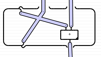
Functors can be represented graphically in string diagrams. This is done by drawing a box around the part of the diagram containing the morphisms that the functor is applied to. This is how it should look like:
        |
  [-------------]
  [  |      |   ]
  [  | (1)  |   ]
  [  \ /    |   ]
  [   +     |   ]
  [   |     |   ]
  [-------------]
         |
Or even more graphically:
And this it what it looks like in Haskell:
                     _id
 |>                  _id
 |>   fd({----}_id…{----------------}_id{---})
 |>   fd(      _id…                  _id     )
 |>   fd(      _id…  (_const 1)…     _id     )
 |>   fd(      _id…  _id…            _id     )
 |>   fd(       (_plus)…             _id     )
 |>   fd(         _id…               _id     )
 |>   fd({-------}_id…{-------------}_id{---})
 |>                        _id
 |>                        _id
Which functor should be applied here follows from the type of the identity morphism in the first line.
Here is an example for the list formation functor with a few additional functor operations that I'm going to explain shortly:
test2 :: [(Int, [Char])]
test2 = cnCurry $ map fromCN . unsingleton . dataFlow
  (
       (                                    monId                           )
    |> (               (mc_list [1,2,3])                                    )
    |> (                         _id                                        )
    |> (                          _id…           (mc_list "aM")             )
    |> (                           _id…                   _id               )
    |> (         fd({-------}_id{--------------------})…    _id             )
    |> (         fd(         _id                      )…     _id            )
    |> (         fd(         _id                      )…     _id            )
    |> (         fd(        _dup…      (mc 1)         )…      _id           )
    |> (         fd(     _id…  _id…      _id          )…      _id           )
    |> (         fd(     _id…   _id…     _id          )…     _id            )
    |> (         fd(     _id…     _id…  _id           )…    _id             )
    |> (         fd(      _id…      _plus             )…    _id             )
    |> (         fd(      _id…      _id               )…   _id              )
    |> (         fd(        _id…   _id…    (mc 2)     )<×>_id               )
    |> (         fd(           _mult…      _id…       _id )                 )
    |> (         fd(              _id…     _id…     _id    )                )
    |> (         fd(              (mc2_1 div)…     _id      )               )
    |> (         fd(                  _id…         _id       )              )
    |> (         fd(                  _id…         _id         )            )
    |> (         fd(                   _id…         _id          )          )
    |> (         fd(                    _id…         _id          )         )
    |> (         fd(                      _id…       _id           )        )
    |> (         fd( (mc_list [2,6])…       _id…    (mf fromEnum)   )       )
    |> (         fd(            _id…          _id…  _id             )       )
    |> (         fd(              _id…          _plus               )       )
    |> (        fd(                 _id…        (mf toEnum)         )       )
    |> (       fd(     fd({---}_id{-------})…   (_id::Typ DF Char)  )       )
    |> (      fd(     fd(      _id          )…     _id             )        )
    |> (     fd(     fd(     _id             )…   _id             )         )
    |> (     fd(     fd(    _id              )<×>_pure           )          )
    |> (     fd(     fd(  _id…   (mc 3)…        _id )           )           )
    |> (     fd(     fd(  _id…    _id…          _id  )         )            )
    |> (     fd(    fd(   _id…    _id…          _id   )       )             )
    |> (     fd(    fd(    _id…  _id…           _id    )     )              )
    |> (     fd(    fd(      _plus…             _id     )   )               )
    |> (      fd(   fd(       _id…               _id     ) )                )
    |> (      join|>fd(       _id…                _id     )                 )
    |> (         fd(      (_id::Typ DF Int)…       _id     )                )
    |> (         fd(          _id…                  _id     )               )
    |> (         fd(          _dup…                   _id    )              )
    |> (         fd(       _id…  _id…                  _id    )             )
    |> (         fd(     _id…     (mf fromIntegral)…   _id     )            )
    |> (         fd(    _id…        _id…               _id     )            )
    |> (         fd(    _id…  (_id::Typ DF Integer)…  _id      )            )
    |> (         fd(     _id…         _id…           _id       )            )
    |> (         fd(       _id…       _id…           _id       )            )
    |> (         fd(        _id…   (mc2_1 genericReplicate)    )            )
    |> (         fd(         _id…          _id                 )            )
    |> (         fd(         _id…          _id                 )            )
    |> (         fd({--------}_id…{------}_id{----------------})            )
    |> (                            _id                                     )
    |> (                            _id                                     )
    |> (                            _id                                     )
  )
Again, we trace from top to bottom what happens to the data. In the beginning, these are again just the empty tuple. Then a list of whole numbers is generated:
       (                                    monId                           )
    |> (               (mc_list [1,2,3])                                    )
    |> (                         _id                                        )
The data are now [1, 2, 3]. Another list is introduced, this time a list of Unicode characters:
    |> (                          _id…           (mc_list "aM")             )
    |> (                           _id…                   _id               )
The data are now ([1,2,3], ['a','M']). Now we open
one of the two functored objects in order to be able to manipulate the list elements:
    |> (         fd({-------}_id{--------------------})…    _id             )
    |> (         fd(         _id                      )…     _id            )
This does not change the data, since a functor, applied to an identity morphism, must yield another identity morphism. But now we can specify inside the functor brackets what functions should be applied to each element of the list:
    |> (         fd(         _id                      )…     _id            )
    |> (         fd(        _dup…      (mc 1)         )…      _id           )
    |> (         fd(     _id…  _id…      _id          )…      _id           )
    |> (         fd(     _id…   _id…     _id          )…     _id            )
    |> (         fd(     _id…     _id…  _id           )…    _id             )
    |> (         fd(      _id…      _plus             )…    _id             )
The data are now ([(1,2),(2,3),(3,4)], ['a','M']). Next the two lists are multiplied
(operator <×>).
This means that every element of the first list is combined with each element of the other list into a tuple.
Besides that, In the same line, a 2 is inserted into each list element:
|> ( fd( _id… _id… (mc 2) )<×>_id )
The data are now [(1,2,2,'a'),(1,2,2,'M'),(2,3,2,'a'),(2,3,2,'M'),(3,4,2,'a'),(3,4,2,'M')].
In the graphical (non-Haskell) notation, one would simply merge the functor frames:
  [ | |      ]    |
  [ | |      ]    |
  [ | |      ]   [---]
  [ | |  (2) ]___[ | ]
  [ | |   |       /  ]
  [ | |   |      /   ]
A functor that allows this operation (and respects a few other rules) is called a monoidal functor.
Here comes a bit of arithmetic:
    |> (         fd(           _mult…      _id…       _id )                 )
    |> (         fd(              _id…     _id…     _id    )                )
    |> (         fd(              (mc2_1 div)…     _id      )               )
    |> (         fd(                  _id…         _id       )              )
    |> (         fd(                  _id…         _id         )            )
    |> (         fd(                   _id…         _id          )          )
    |> (         fd(                    _id…         _id          )         )
The data are now [(1,'a'),(1,'M'),(3,'a'),(3,'M'),(6,'a'),(6,'M')].
A list is inserted into each element, and the Unicode code point of the characters is determined:
    |> (         fd(                      _id…       _id           )        )
    |> (         fd( (mc_list [2,6])…       _id…    (mf fromEnum)   )       )
    |> (         fd(            _id…          _id…  _id             )       )
The data are now [([2,6],1,97),([2,6],1,77),([2,6],3,97),([2,6],3,77),([2,6],6,97),([2,6],6,77)].
The second and third element of each tuple are added and the result should be converted back into a character.
    |> (         fd(              _id…          _plus               )       )
    |> (        fd(                 _id…        (mf toEnum)         )       )
However, the Haskell function toEnum that converts integers to elements of enumeration types
is too generic. We have to specify which enumeration type (namely, Char) the result should belong to.
This works as follows:
(DF is an abbreviation for the category, DataFlow):
    |> (       fd(     fd({---}_id{-------})…   (_id::Typ DF Char)  )       )
    |> (      fd(     fd(      _id          )…     _id             )        )
The data are now [([2,6],'b'),([2,6],'N'),([2,6],'d'),([2,6],'P'),([2,6],'g'),([2,6],'S'].
On the side, the functor brackets for the inner list were opened.
Next, we want to combine the characters and the numbers into pairs.
If the characters were wrapped into singleton lists, we could multiply the lists as we did before to reach that goal.
The list functor is an
applicative functor,
therefore it has an operation pure
that maps objects to functored objects in a canonical way.
For lists in Haskell, this operation happens to be the wrapping of an element into a singleton list.
(It could have been different. Another reasonable choice would be making an infinite list with all equal elements.)
Thus we apply _pure to the characters and multiply
the [2,6] with the result:
    |> (     fd(     fd(     _id             )…   _id             )         )
    |> (     fd(     fd(    _id              )<×>_pure           )          )
The data are now [[(2,'b'),(6,'b')],[(2,'N'),(6,'N')],[(2,'d'),(6,'d')],[(2,'P'),(6,'P')],[(2,'g'),(6,'g')],[(2,'S'),(6,'S')]].
Now each of the numbers is increased by 3:
    |> (     fd(     fd(  _id…   (mc 3)…        _id )           )           )
    |> (     fd(     fd(  _id…    _id…          _id  )         )            )
    |> (     fd(    fd(   _id…    _id…          _id   )       )             )
    |> (     fd(    fd(    _id…  _id…           _id    )     )              )
    |> (     fd(    fd(      _plus…             _id     )   )               )
The data are now [[(5,'b'),(9,'b')],[(5,'N'),(9,'N')],[(5,'d'),(9,'d')],[(5,'P'),(9,'P')],[(5,'g'),(9,'g')],[(5,'S'),(9,'S')]].
The list functor is a
monad.
This means that in addition to the operations of an applicative functor it has another operation, the join
operation:
Two nested applications of the functor can be
naturally transformed to a single application.
For lists, this operation is the concatenation of the elements (that are themselves lists): A list of lists thus becomes a simple list.
    |> (      fd(   fd(       _id…               _id     ) )                )
    |> (      join|>fd(       _id…                _id     )                 )
The data are now [(5,'b'),(9,'b'),(5,'N'),(9,'N'),(5,'d'),(9,'d'),(5,'P'),(9,'P'),(5,'g'),(9,'g'),(5,'S'),(9,'S')].
Now the numbers are duplicated, so that the first copy becomes an Int value and the second becomes an
Integer value. Why? No particular reason. Perhaps to test the interaction between my notation and the type checker.
    |> (         fd(      (_id::Typ DF Int)…       _id     )                )
    |> (         fd(          _id…                  _id     )               )
    |> (         fd(          _dup…                   _id    )              )
    |> (         fd(       _id…  _id…                  _id    )             )
    |> (         fd(     _id…     (mf fromIntegral)…   _id     )            )
    |> (         fd(    _id…        _id…               _id     )            )
    |> (         fd(    _id…  (_id::Typ DF Integer)…  _id      )            )
    |> (         fd(     _id…         _id…           _id       )            )
The data are now [(5,5,'b'),(9,9,'b'),(5,5,'N'),(9,9,'N'),(5,5,'d'),(9,9,'d'),(5,5,'P'),(9,9,'P'),(5,5,'g'),(9,9,'g'),(5,5,'S'),(9,9,'S')].
However, you don't see a difference between Int and Integer values here.
We use the second number of each triple to turn the character into a string of this many equal characters:
    |> (         fd(       _id…       _id…           _id       )            )
    |> (         fd(        _id…   (mc2_1 genericReplicate)    )            )
    |> (         fd(         _id…          _id                 )            )
The end result is [(5,"bbbbb"),(9,"bbbbbbbbb"),(5,"NNNNN"),(9,"NNNNNNNNN"),(5,"ddddd"),(9,"ddddddddd"),(5,"PPPPP"),(9,"PPPPPPPPP"),(5,"ggggg"),(9,"ggggggggg"),(5,"SSSSS"),(9,"SSSSSSSSS")].
To conclude, we close
the functor box to indicate that we are done manipulating the list elements:
    |> (         fd(         _id…          _id                 )            )
    |> (         fd({--------}_id…{------}_id{----------------})            )
    |> (                            _id                                     )
    |> (                            _id                                     )
    |> (                            _id                                     )
As I already mentioned, (T ->) is a functor for every parameter type T.
We can use this to define anonymous functions. Here is an example:
test4 :: Num a =>  (a, a)
test4 = cnCurry $ fromCN . dataFlow
 (monId
  |>  (    (_const 19)                                        )
  |>  (       _id                                             )
  |>  (       _id…               (_const _id)                 )
  |>  (       _id…         fd({---}_id{----------------})     )
  |>  (       _id…         fd(     _id                  )     )
  |>  (       _id…         fd(     _id                  )     )
  |>  (       _id…         fd(     _id…   (_const 4)    )     )
  |>  (       _id…         fd(      _id…  _id           )     )
  |>  (        _id…        fd(        _plus             )     )
  |>  (        _id…        fd(         _id              )     )
  |>  (        _id…        fd(         _id              )     )
  |>  (        _id…        fd({------}_id{-------------})     )
  |>  (        _id…       _id                                 )
  |>  (         _id…      _id                                 )
  |>  (         _id…       _id                                )
  |>  (         _id…        (_dup)                            )
  |>  (          _id…     _id… _id…       (_const 5)          )
  |>  (          _id…    _id…    _id…   _id                   )
  |>  (           _id…  _id…       (apply)                    )
  |>  (             _swap…           _id                      )
  |>  (           _id…  _id…          _id                     )
  |>  (          _id…    _id…         _id                     )
  |>  (            (apply)…            _id                    )
  |>  (             _id…               _id                    )
  |>  (             _id…               _id                    )
 )
First, the morphism (_const _id) generates an identity function.
Then a functor box is opened.
Inside, each line is a description of what to do with the return value of the respective previous line:
First the value is paired with the constant 4, then the two elements of the pair are added.
The finished function thus is the function that adds 4 to its argument.
Then this function is duplicated and each copy is applied to a number.
The application may be imagined as the argument being transported upwards in the left boundary of the functor box, turning around at
(_const _id) and going into the interior of the box, where it is processed. The result is transported down till it
reaches the location where the function was invoked.
The view that the argument runs upwards hidden in the left boundary of the functor box isn't even that devious.
To wit, the functor (T ->) arises from the
bifunctor
(->) by fixing an object as the first argument of the bifunctor.
A bifunctor is a functor from the Cartesian product of two categories into a target category. In out case, the second category and the target category
are the category of data flow graphs, and the first category is its dual category, that is the category where all morphisms are reversed.
The morphisms of this Cartesian product might be denoted like this:
f ]+[ g
Together with the bifunctor brackets this becomes two compartments
:
[ f ]+[ g ]
In Haskell, we may write it like this:
f2( f )( g )
With this bifunctor, you can do the following:
test12 ::(Num a)=> a -> a
test12 = (unsingleton.)$cnCurry $ dataFlow
 (   (                                                         _id      )
  |> (                                                         _id      )
  |> (                                                          _id     )
  |> (                       (_const _id)…                       _id    )
  |> (  f2({----------------}_id )( _id{--------------------})…   _id   )
  |> (  f2(                _id   )(   _id                    )…   _id   )
  |> (  f2(              _id     )(    _id                   )…   _id   )
  |> (  f2(            _id       )(     _id…    (mc 4)       )…   _id   )
  |> (  f2(       (Dual _mult)   )(      _id…  _id           )…   _id   )
  |> (  f2(       _id…     _id   )(        _plus             )…   _id   )
  |> (  f2( (Dual(mc 2))…  _id   )(         _id              )…   _id   )
  |> (  f2(               _id    )(         _id              )…   _id   )
  |> (  f2({------------}_id{---})({------}_id{-------------})…   _id   )
  |> (                          _id…                             _id    )
  |> (                            _id…                          _id     )
  |> (                              _id…                       _id      )
  |> (                                _id…                    _id       )
  |> (                                  _id…                 _id        )
  |> (                                    _id…              _id         )
  |> (                                      _id…           _id          )
  |> (                                        _id…        _id           )
  |> (                                          _id…     _id            )
  |> (                                            _id…  _id             )
  |> (                                             (apply)              )
  |> (                                              _id                 )
  |> (                                              _id                 )
  |> (                                              _id                 )
 )
Here the argument is multiplied by 2 on its way up.
Because the left compartment contains morphisms of the dual category, the left subdiagram is flipped on its head.
For the morphisms in the compartment, vertical composition is defined the other way round.
In order to have two different meanings of the vertical composition, I had to give a newtype definition
for the dual morphisms (newtype Dual f=Dual f).
The morphisms then must be wrapped into this new type, either by always writing e.g. Dual _mult instead of _mult, or, in
the case of general category generating morphisms like _id and _swap, as part of a category type class.
The (left partial) trace of a morphism can be defined graphically as follows:
        |   |
 /¯\    |   |
 |  examplomorphism
 \_/     |
         |
The leftmost factor of the target object is bent around to the top and taken as leftmost factor of the source object. But this bending-up only works if the category has dual objects, like for example the category of finite dimensional vector spaces with the tensor product, where the trace is the ordinary trace of a tensor. In the category of data flow graphs, however, there are no dual objects. A hypothetical dual object T* would be something like the type of a promise to deliver later exactly one value of type T. Such a dual value would need to be protected from duplication and deletion to ensure that exactly one value is supplied. But that cannot be enforced if dual objects are to be first class members of the category.
Functors can provide a workaround, as I demonstrate for the category of data flow graphs with the (T ->) functor:
test6 :: Num fr => fr -> fr -> fr
test6 = cnCurry $ unsingleton . dataFlow
  ((                       _id …        _id         )
  |>  (                    _id…         _id         )
  |>  (                    _id…         _id         )
  |>  (                    _id…         _id         )
  |>  (             ({---------}packC{---------})   )
  |>  (           fd(       _id…       _id      )   )
  |>  (  param <| fd(       _id…      _id       )   )
  |>  (  fd(   _id…         _id…      _id       )   )
  |>  (  fd(     _id…     _id…      _id         )   )
  |>  (  fd(        (_swap)…      _id           )   )
  |>  (  fd(     _id…     _id…  _id             )   )
  |>  (  fd(    _id…        _plus               )   )
  |>  (  fd(   _id…         _id                 )   )
  |>  (  trace |> fd(       _id                 )   )
  |>  (           fd(       _id                 )   )
  |>  (           fd(       _id                 )   )
  |>  (           ({-------}unpack{------------})   )
  |>  (                     _id                     )
 )
The morphism whose trace is taken has three inputs and two outputs:
      (          _id…     _id…      _id             )
  |>  (             (_swap)…      _id               )
  |>  (          _id…     _id…  _id                 )
  |>  (         _id…        _plus                   )
  |>  (        _id…         _id                     )
Its trace has just two inputs and one output. To calculate the trace,
both inputs are first wrapped into a nullary function using packC.
The the function param is applied to the functored object.
The line
|> ( param<| fd( _id… _id ) )
is actually two lines, as <| is the vertical composition, only with swapped parameters.
For aesthetic reasons I have written both on the same line.
The function param transforms a function object so that a parameter is added to the left.
So here, a function of type ()->(a, b) is transformed into a function of type (p)->(p, a, b).
Now the morphism whose trace we want to obtain can be applied under the functor.
Then the function trace is applied to the function object.
In Haskell syntax, it is defined as follows (simplified):
trace' :: ((p :*: a) -> (p :*: b)) -> (a -> b)
trace' f a = b where
  (p :*: b) = f (p :*: a)
--
trace = mf trace'
Thus, the function f gets fed a part p of its return value as a part of its arguments.
This works because Haskell has
Lazy Evaluation.
Afterwards, the result must be unwrapped from the (()->) functor, which is done with unpack in my notation.
The trace that we get this way is simply a morphism that performs the addition of two numbers in a roundabout way:
The first argument takes an extra turn before it is added to the second.
Because the value is hidden in the left wall of the functor box on its way up, it is protected from uncontrolled deletion and duplication; dual objects are not needed.
Can we do something useful with this? Yes, namely defining recursive functions.
This is how it works:
Lead a wire of _ids, which will later conduct the recursive function as its value, into the functor box of the function definition.
There you can then let the function call itself (with apply). If the definition proper is done, you close the the functor box and duplicate
the function just defined with _dup.
Then draw a functor box around everything to take the trace. Thus one of the two copies of the recursive function
is lead back up using trace and param (or (_const _id)) so that it is available
for its own definition. The other copy is lead out of the functor box (which after application of trace refers just to the (()->) functor)
using unpack.
Here is an example that computes the infinite list of all natural numbers:
test10 :: Num a => [a]
test10 = cnCurry $ unsingleton . dataFlow
 (    (       (_const _id)                                    )
   |> (     fd({------------------}_id{-----------------})    )
   |> (     fd(                    _id                   )    )
   |> (     fd(          ({-------}packC{-----------})   )    )
   |> (     fd( param<|fd(         _id               )   )    )
   |> (     fd( fd(     _id…       _id               )   )    )
   |> (     fd( fd(     _dup…      _id               )   )    )
   |> (     fd( fd(   _id… _id…    _id               )   )    )
   |> (     fd( fd(  _id…   _id…  _id…   (_const 1)  )   )    )
   |> (     fd( fd(  _id…     _swap…      _id        )   )    )
   |> (     fd( fd(  _id…   _id…   _id…  _id         )   )    )
   |> (     fd( fd(  _id…    _id…    _plus           )   )    )
   |> (     fd( fd(  _id…     _id…  _id              )   )    )
   |> (     fd( fd(  _id…       apply                )   )    )
   |> (     fd( fd(  _id…        _id                 )   )    )
   |> (     fd( fd(   _id…      _id                  )   )    )
   |> (     fd( fd(    (mc2_1 (:))                   )   )    )
   |> (     fd( fd(        _id                       )   )    )
   |> (     fd( fd({------}_id{---------------------})   )    )
   |> (     fd(                  _id                     )    )
   |> (     fd(               _dup                       )    )
   |> (     fd(           _id…   _id                     )    )
   |> (     fd(         _id…     _id                     )    )
   |> (     fd(      _id…        _id                     )    )
   |> (     trace|>fd(           _id                     )    )
   |> (     fd(                  _id                     )    )
   |> (     ({-----------------}unpack{-----------------})    )
   |> (                _id                                    )
   |> (                _id…   (_const 0)                      )
   |> (                 _id…   _id                            )
   |> (                    apply                              )
   |> (                    _id                                )
 )
Another example of a recursive function is the fixed-point combinator. In ordinary Haskell it is defined thus:
fix :: (t -> t) -> t
fix f = f (fix f)
or
fix f = x where x = f x
For any given function it calculates a value that is not changed by that function.
One can use the fixed-point combinator to define recursive functions without the function definition being syntactically recursive.
To define a recursive function f::x->y, first define a function f'::r->x->y by replacing in the recursive definition of f
every occurrence of f with the first parameter of f'. The function f then is the fixed point of
f', i.e. (fix f'). This is how the fixed-point combinator looks as a string diagram:
_fix :: DataFlow   (DataFlow (a :*: ()) (a :*: ())  :*:  ())   (a :*: ())
_fix = (                     _id             )
  |>   (           ({------}packC{-----})    )
  |>   (  param<|fd(         _id        )    )
  |>   (  fd(     _id…      _id         )    )
  |>   (  fd(       _id…  _id           )    )
  |>   (  fd(         _swap             )    )
  |>   (  fd(       _id…  _id           )    )
  |>   (  fd(      _id…   _id           )    )
  |>   (  fd(         apply             )    )
  |>   (  fd(          _id              )    )
  |>   (  fd(          _id              )    )
  |>   (  fd(          _dup             )    )
  |>   (  fd(       _id… _id            )    )
  |>   (  fd(     _id…    _id           )    )
  |>   (  trace|>fd(       _id          )    )
  |>   (         fd(       _id          )    )
  |>   (         ({------}unpack{------})    )
  |>   (                    _id              )
  |>   (                    _id              )
And in this way you can use it to generate the list of all natural numbers:
test7 :: Num a => [a]
test7 = cnCurry $ unsingleton . dataFlow
 (    (       (_const _id)                                    )
   |> (     fd({------------------}_id{-----------------})    )
   |> (     fd(                    _id                   )    )
   |> (     fd(          ({-------}packC{-----------})   )    )
   |> (     fd( param<|fd(         _id               )   )    )
   |> (     fd( fd(     _id…       _id               )   )    )
   |> (     fd( fd(     _dup…      _id               )   )    )
   |> (     fd( fd(   _id… _id…    _id               )   )    )
   |> (     fd( fd(  _id…   _id…  _id…   (_const 1)  )   )    )
   |> (     fd( fd(  _id…     _swap…      _id        )   )    )
   |> (     fd( fd(  _id…   _id…   _id…  _id         )   )    )
   |> (     fd( fd(  _id…    _id…    _plus           )   )    )
   |> (     fd( fd(  _id…     _id…  _id              )   )    )
   |> (     fd( fd(  _id…       apply                )   )    )
   |> (     fd( fd(  _id…        _id                 )   )    )
   |> (     fd( fd(   _id…      _id                  )   )    )
   |> (     fd( fd(    (mc2_1 (:))                   )   )    )
   |> (     fd( fd(        _id                       )   )    )
   |> (     fd( fd({------}_id{---------------------})   )    )
   |> (     fd(                  _id                     )    )
   |> (     fd({----------------}_id{-------------------})    )
   |> (                _id                                    )
   |> (                _fix…   (_const 0)                     )
   |> (                 _id…   _id                            )
   |> (                   apply                               )
   |> (                    _id                                )
 )
When may this mechanism of forming the trace be generalized to other traced monoidal categories?
In general, trace formation is defined as a family of functions on the morphisms, but isn't necessarily representable itself as a morphism like
trace.
An important prerequisite for that to work is that the category is
closed, which essentially means that the types of morphisms are again objects in the category.
Only due to this could we just wrap a morphism m from (P × A) to (P × B) in an object under the
(P × A →) functor and then take the trace of the functored object using trace.
We also need a possibility to lead the inputs (of type A) for the trace into the interior of the functor box, as I have done with
packC.
For this, a closed category C needs a
unit object I,
so than one can form a packC-like morphism from the object A to the object (I → A).
This morphism is given by a natural transformation from the identity functor to the (I →) functor, which should be invertible
in order to be able to apply an unpack-like morphism from (I → B) to B in the end,
to get as the overall result of the trace formation a morphism from A to B.
The unit object is not necessarily identical to the neutral element of the monoidal product,
for example in the category of control flow graphs (see above).
If there is a unit object, one may talk about elements of an object O – these are given by the morphisms from I to O.
And of course morphisms have to exist in the category C that take the role of
param and trace.
Alternatively to morphisms analogous to param, packC and unpack, in a
closed monoidal category
morphisms analogous to (_const id) and apply may be used: First comes a morphism from the monoidal identity object
to the object ((P A) → (P A)) that generates the identity morphism of (P A), wrapped into an object,
then comes the image of m under the ((P A) →) functor followed by trace. Finally the apply-like morphism is used
to connect the morphism that is wrapped into an element of (A → B) to the identity morphism of A which
the whole time over stood to the right of the other morphisms.
The monoidal product does not necessarily have to be Cartesian for
apply to exist as a morphism from ((A → B) A) to B;
although it doesn't work in the category of control flow graphs (with disjoint union for the monoidal product), in the category of finite dimensional vector spaces
and linear maps with the tensor product, apply exists as a linear map from
(A* ⊗ B) ⊗ A to B, given by the appropriate
tensor contraction.
It does not work with control flow graphs because, although this category is closed and monoidal, the two structures are not compatible since the unit object
needed for closedness is not the same as the unit object of the monoidal product and the (⊕ X) functor is not
adjoint to the (X →) functor.
Nevertheless there is a notion of trace in the category of control flow graphs, which corresponds to the formation of loops.
As the morphisms here are functions and all function types occur as objects in the category, it should be possible to express traces, similarly to how it is done
in the category of data flow graphs, with param and trace.
The trace function must be defined in a markedly different way, shown here for a morphism examplomorphism that
maps the disjoint union of three data types to the disjoint union of two data types:
                                           |        |
                                  .        |        |
(_const examplomorphism)          |        |        |
   |                       =   (trace' examplomorphism)
 trace                                       |
   |                                         |
Here, . is a morphism that adds a summand to the disjoint union of data types,
and trace' is defined recursively as
|       |      |             |   |  |
(trace' morphism) =          morphism
        |                    |      |
        |                    | . .  |
        |                    | | |  |
        |         (trace' morphism) |
        |                        |  |
        |                         \/
        |                         |
The morphism \/ maps from the disjoint union of a data type T with itself to the type T by forgetting which summand the value came from.
By the way, the morphisms . and \/ together define a
monoid for every type T:
The morphism . generates a neutral element, and \/ turns two elements of type T into a single one in an associative way.
Other monoids, in the category of data flow graphs, that however are defined only for numeric types, would be
_plus with (_const 0) and _mult with (_const 1).
Before we see the trace operator for the category of control flow graphs in action, we will first take a closer look at how to work with this category in Haskell.
Associated to every _id-wire is a data type. Of several parallel wires, only one can contain data at runtime
because the horizontal composition denotes the disjoint union of data types.
To express something meaningful in this category, we have to be able to describe what should happen to the data.
For this task data flow graphs are better suited. So we need a possibility to embed data flow graphs into the control flow graph.
For this we can use a functor, this time from the category of data flow graphs to the category of control flow graphs.
I have called this functor DFF. Thus, for example, the data type of a pair of integers in the category of control flow graphs
would be DFF (Int :*: Int :*: ()). To access the elements in the pair, open a functor box and write a data flow graph inside.
An important morphism in the category of control flow graphs is the the one for branching the control flow.
I have called it _if.
As input it expects a DFF-functored tuple of type DFF (Bool :*: rest) (for some typle type rest)
and turns it into an element of the disjoint union of DFF rest with itself: If the leftmost element of the input tuple
has the value True, the remaining part of the data (the one with type DFF rest) is marked as belonging to the left summand of the disjoint union,
otherwise it is marked as belonging to the right summand.
Another important morphism is the one for merging control flows, which I called \/ above and _codup (coduplication) in Haskell.
Here is an example the demonstrates _if, _codup and the DFF functor:
collatzStep =
 (    (                 _id                                                   )
   |> (                 _id::Typ ControlFlow (DFF(Integer:*:[Integer]:*:()))  )
   |> (                   _id                                                 )
   |> (                     _id                                               )
   |> (                 fd({-----------}_id…{-----------}_id )                )
   |> (                 fd(             _id…             _id )                )
   |> (                 fd(            (_dup)…           _id )                )
   |> (                 fd(           _id… _id…          _id )                )
   |> (                 fd(         _id…    (_dup)…      _id )                )
   |> (                 fd(       _id…    _id…   _id…    _id )                )
   |> (                 fd(     (_even)…   _id…   (mc2_1 (:)))                )
   |> (                 fd(       _id…      _id…        _id  )                )
   |> (                 fd({-----}_id…{-----}_id…{------}_id )                )
   |> (                               _id                                     )
   |> (                               _id                                     )
   |> (                               _id                                     )
   |> (                              (_if)                                    )
   |> (                            _id… _id                                   )
   |> (                          _id…    _id                                  )
   |> (                        _id…       _id                                 )
   |> (    fd({---}_id…{--------}_id )…    fd({---}_id…{-----------}_id )     )
   |> (    fd(    _id…           _id )…    fd(     _id…             _id )     )
   |> (    fd(   _id…   (mc 2)…  _id )…    fd(     _id…   (mc 3)…   _id )     )
   |> (    fd(   _id…  _id…      _id )…    fd(     _id…   _id…      _id )     )
   |> (    fd(     (_div)…       _id )…    fd(       (_mult)…       _id )     )
   |> (    fd(      _id…         _id )…    fd(     _id…             _id )     )
   |> (    fd({----}_id…{-------}_id )…    fd(     _id…  (mc 1)…    _id )     )
   |> (                  _id…              fd(     _id…  _id…       _id )     )
   |> (                    _id…            fd(       _plus…         _id )     )
   |> (                      _id…          fd(        _id…          _id )     )
   |> (                        _id…        fd({------}_id…{--------}_id )     )
   |> (                          _id…         _id                             )
   |> (                            _id…     _id                               )
   |> (                              (_codup)                                 )
   |> (                                _id                                    )
 )
The input is a pair consisting of an integer and a list of integers.
In the first functor box the first element of the pair is triplicated. The leftmost copy is tested if it is an even number.
The rightmost copy is appended to the front of the list.
The result is a triple consisting of a truth value, the integer and the augmented list.
Then the functor box is closed and the triple is passed to the morphism _if.
Then, depending on whether the truth value was True or False, either the left or the right part of the following is executed.
In the left part (when the number is even), the number is divided by 2, and in the right part, when it is uneven, it is
multiplied by 3 and incremented by 1. Then the two alternate control flows are merged again.
This control flow diagram calculates a single step of the generation of a
Collatz sequence.
What about the calculation of the complete sequence for a given number?
(Here I'm going to assume that the Collatz conjecture is true, so we can terminate the calculation as soon as the sequence reaches 1.)
For this we have to make a loop, and that is done with param and trace. Here is the necessary code:
collatz n = unsingleton . unDFF . fromLeft $ collatz' (Left (DFF (n:*:()))) where
  fromLeft (Left a) = a
  collatz' = controlFlow
    (    (                             _id                    )
      |> (                             _id                    )
      |> (            ({-------------}packC{--------------})  )
      |> (          fd(                _id                 )  )
      |> (          fd( fd({---}_id{----------------})     )  )
      |> (          fd( fd(     _id                  )     )  )
      |> (          fd( fd(     _id…      (mc [])    )     )  )
      |> (          fd( fd(     _id…        _id      )     )  )
      |> (          fd( fd({---}_id…{------}_id{----})     )  )
      |> (          fd(                _id                 )  )
      |> (   param<|fd(              _id                   )  )
      |> (   fd(     _id…          _id                     )  )
      |> (   fd(       _id…      _id                       )  )
      |> (   fd(         _id…  _id                         )  )
      |> (   fd(          _codup                           )  )
      |> (   fd(            _id                            )  )
      |> (   fd(            _id                            )  )
      |> (   fd(         (collatzStep)                     )  )
      |> (   fd(              _id                          )  )
      |> (   fd(     fd({-------------}_id…{------}_id )   )  )
      |> (   fd(     fd(               _id…        _id )   )  )
      |> (   fd(     fd(  (mc 1)…      _dup…       _id )   )  )
      |> (   fd(     fd(   _id…     _id…  _id…     _id )   )  )
      |> (   fd(     fd(   (mc2_1 (/=))…   _id…    _id )   )  )
      |> (   fd(     fd(       _id…       _id…     _id )   )  )
      |> (   fd(     fd({-----}_id…{-----}_id…{---}_id )   )  )
      |> (   fd(                     _id                   )  )
      |> (   fd(                     _id                   )  )
      |> (   fd(                    (_if)                  )  )
      |> (   fd(                  _id… _id                 )  )
      |> (   fd(                _id…   _id                 )  )
      |> (   fd(              _id…     fd( _id…{---}_id )  )  )
      |> (   fd(            _id…       fd( _id…     _id )  )  )
      |> (   fd(          _id…         fd(  (mc2_1 (:)) )  )  )
      |> (   fd(        _id…           fd(      _id     )  )  )
      |> (   fd(      _id…             fd( (mf reverse) )  )  )
      |> (   trace|>fd(                fd(      _id     )  )  )
      |> (          fd(                fd({----}_id{---})  )  )
      |> (          fd(                _id                 )  )
      |> (          fd(                _id                 )  )
      |> (            ({-------------}unpack{-------------})  )
      |> (                             _id                    )
      |> (                             _id                    )
    )
The input is a DFF-functored 1-tuple containing a whole number.
This is wrapped into the (()->) functor using packC and subsequently augmented by a second element – an empty list.
I could also have first added the empty list and then wrapped it into the functor; it doesn't matter.
Then a parameter is added to the function. We have to bear in mind that multi-parameter functions in the category of control flow graphs get passed a single argument
when they are called; all other parameters stay empty. Which parameter is filled
decides where in the function with multiple entry points the control flow begins.
The control flow now has two alternate possibilities: either it comes from a previous iteration of the loop (left) or we have just entered the loop (right).
Because we do not care about that for the upcoming iteration of the loop, the two control flows are merged with _codup.
Then a single Collatz step is executed (collatzStep, see above).
The result is again a pair of an integer and a list of integers. The integer is compared to 1 for testing the termination condition.
This splits the control flow into two alternatives: If the number wasn't 1, it jumps back to the beginning of the loop via trace.
If the number however was 1, the loop is exited.
The 1 is appended to the front of the list and the list is reversed, to get prettier output.
Afterwards (I could also have done if before) the list is unwrapped from the (()->) functor.
It is quite fun to be able to make executable two-dimensional diagrams out of Haskell source code, but in the long run it is a bit arduous, at least if you endeavor to make them look good. A graphical editor would be nice to have. I have begun writing such an editor. With it I made the two images in this article. But it can neither represent monoidal functors and monads nor generate executable code yet. What also would be nice: Performing algebraic manipulations of morphisms and functors directly in the string diagram with the mouse. At the end of these slides there is an example for a proof based on the graphical manipulation of string diagrams. A program to generate such graphical proofs might also be interesting for (didactics of) mathematics.
It is difficult to teach the Haskell type system how to compose morphisms and functors. Some operations I could not define in that generality in which I would have liked to. Perhaps it would be better to use a language specifically constructed for this, whose type system is construed with monoidal categories in mind. Then one could also use a prettier notation. I already have ideas on how to represent types as string diagrams themselves.
The monad operations join
and pure
are just two examples of
natural transformations.
In general, natural transformations are represented in string diagram notation as nodes in the side walls of functor boxes which
change the number of side walls and/or the associated functors. Thus there is a syntactical similarity between natural transformations
and ordinary morphisms: Both have inputs and outputs, only that with morphisms these are objects and and with natural transformations
these are functors. Indeed, natural transformations are the 2-morphisms
in the 2-category Cat, whose objects are the (ordinary) 1-categories
and whose 1-morphisms are functors. Similarly to morphisms in a monoidal category, one can both vertically and horizontally compose
the 2-morphisms of a 2-category. The difference is that for horizontal composition it is also required that the source and target objects of the transformed
1-morphisms match. Nevertheless, 2-categories have a string diagram calculus very similar to monoidal categories.
And if we restrict ourselves to endofunctors, that is functors from a category into itself, then the source and target categories
always agree and we even get a proper monoidal category, whose objects are endofunctors and whose monoidal product is given by writing natural
transformations side by side.
In the category of endofunctors, the natural transformations join
and pure
form a monoid.
A monoid in the category of endofunctors is just a monad, what's the problem?
Anyway, it would be interesting if you could compose natural transformations in string diagram notation.
How to realize that in Haskell, I do not know yet. I haven't even tried yet.
param and trace are natural transformations too, or rather components thereof:
In the category of data flow graphs param goes from the functor (T →) to the functor ((P × T) →)∘(P ×) and
trace goes in the other direction,
and in the category of control flow graphs they go between the functor (T →) and the functor ((P ⊕ T) →)∘(P ⊕).
Due to the special role of the monoidal products (×) or (⊕) in these categories it looks as if
a factor of type P was introduced or removed on the interior of the functor box at the natural transformation.
This possibility should also be incorporated when designing a string diagram notation for natural transformations.